|
Session 11
COMPUTATIONAL & MATHEMATICAL METHODS II
Chairman: M. Wolfshtein
NOVEL SPECTRAL AND FINITE ELEMENT METHODS FOR UNSTEADY HEAT TRANSFER PROBLEMS
P. Bar-Yoseph
A bifurcation from steady to oscillatory state of buoyant convective flow in laterally heated rectangular cavities is numerically investigated. The considered flow is defined by the momentum, the continuity and the energy equations in the Boussinesq approximation and the three characteristic parameters: Grashof number Gr, Prandtl number Pr and the aspect ratio of the cavity (length/height) A. Cavities with 4 no-slip boundaries, isothermal vertical boundaries and perfectly insulated horizontal boundaries are considered. Case of a stress-free upper boundary was considered in 1. The analysis is focused on the case of low Prandtl number fluid, in particular Pr=0 and Pr=0.015. The aspect ratio is varied from 1 to 10.
The problem was numerically investigated using the spectral Galerkin method with globally defined basis functions which satisfy all the boundary conditions and the continuity equation. The global formulation of the Galerkin method allows us to decrease the number of degrees of freedom (number of scalar modes in the numerical method), which gives a possibility to investigate consequently steady states, their stability and weakly supercritical states of the flow in the framework of a single model. Results of Galerkin method are verified by solution of the full unsteady Boussinesq problem with the use of the finite volume method. Both numerical techniques are described in detail in 2,3.
The most unexpected result of this study is existence of several branches of steady states. For aspect ratio 4 the existence of 2 different steady states was previously reported 4, namely flow with one main convective vortex and flow with 2 separated vortices. While stability of these known states was studied, other branches steady states flows with 3 and 4 separated vortices were discovered for cavities of larger aspect ratios. Examples of such flows are shown in Figs. 1 and 2. These steady states were calculated first by the Galerkin method and then some of them were reobtained by the finite volume method which approved their existence. Another set of multiple steady states was found for cavities with 1<A<2 and Pr=0 (Fig.3). Initially all the steady flow are symmetric with respect to rotation around the center of the cavity. Lower line between points A and B in Fig.3 corresponds to a steady bifurcation from symmetric to non-symmetric steady state (Fig.4). Upper line between points I and II corresponds to the oscillatory instability of non-symmetric steady states. Region in Gr-A plane where non-symmetric steady states are stable becomes smaller with the increase of the Prandtl number and completely disappears at Pr=0.015.
Other objectives of this study are to compare oscillatory instability at zero and low Prandtl numbers (Pr=0.015) and at large and infinite aspect ratios (A=10 and the infinite fluid layer, A=¥ ). It was found that a similarity between the most unstable perturbations at Pr=0 and 0.015 as a rule does not exist. Such similarity may be found, for example, at A=4 (see Ref.2) for single-vortex steady states. Behavior of steady states at large aspect ratios show some analogies with the infinite layer. Namely, a single-vortex state transforms into a many vortex state and vice versa. These transitions, depending on the aspect ratio and the Prandtl number, may either continuously transform one into another or change abruptly because of instability of one of them. On the other hand, no asymptotic behavior for large A was found for the critical Grashof number and the critical frequency corresponding to the onset of oscillatory instability. The most unsteady perturbations also show that the influence of the confined geometry on the stability of the flow cannot be neglected. This is illustrated in Fig.5 where isolines of the flow at the critical values of parameters are shown together with isolines of the most unstable perturbation of this flow. It is seen that at A=10 the flow has spatially periodic features, as it is expected by the analogy of an infinite fluid layer. On the other hand, the most unstable perturbation has no such features which means that the confined shape of the cavity has an important influence on the onset of the instability.
|
Fig. 1. Examples of different branches of steady state flows. Pr=0.015.
(a) A=3.5, Gr=6.4´ 106,
(b) A=5, Gr=4.25´ 106,
(c) A=7, Gr=2.85´ 106.
|
Fig. 2. Multiple steady state flows at Pr=0, A= 7, Gr=8.8´ 104. All three steady states are stable
|
|
|
|
|
Fig. 3. Stability diagram for Pr=0, 1£ A£ 3.5. |
Fig. 4. Examples of symmetric and non-symmetric steady state flows. Pr=0.
(a) A=1.5, Gr=2´ 105,
(b) A=1.57, Gr=2.3´ 105,.
|
|
Fig. 5. Streamlines (solid lines), isotherms (solid lines) and the corresponding most unstable perturbation (dash lines). A=10, Pr=0.015, Gr=6.2´ 106
|
ACKNOWLEDGEMENT
This research was supported by the German-Israeli Foundation for Scientific Research and Development, grant No.I-284.046,10/93.
REFERENCES
- Gelfgat A.Yu., Bar-Yoseph P.Z. and Yarin A.L. Numerical Investigation of Hopf Bifurcation Corresponding to Transition From Steady to Oscillatory State in a Confined Convective Flow. Proc. of the 1996 ASME Fluids Engineering Division Summer Meeting, FED - vol.237, pp 369-374, 1996.
- Gelfgat A.Yu. and Tanasawa I. Numerical Analysis of Oscillatory Instability of Buoyancy Convection with the Galerkin Spectral Method. Numerical Heat Transfer. Part A., Vol. 25, pp 627-648, 1994.
- Gelfgat A.Yu., Bar-Yoseph P.Z. and Solan A. . Stability of Confined Swirling Flow with and without Vortex Breakdown. Journal of Fluid Mechanics, Vol. 311, pp 1-36, 1996.
- Roux B. (ed.). Numerical Simulation of Oscillatory Convection in Low-Pr Fluids: A GAMM Workshop. Notes on Numerical Fluid Mechanics, Vol. 27, 1989.
SIMULATION OF BUBBLE MOTION IN BENARD CELLS BY SPECTRAL METHODS
Ilker Tari* ,
Andrew Tangborn+
Yaman Yener*
* Mechanical, Industrial and Manufacturing Eng. Dept., Northeastern University, Boston, MA.
+ CIRES, University of Colorado, Boulder, CO.
The study of the interaction of bubble motion with fluid motion in laminar and turbulent flows is of special interest not only for the understanding of the underlying physics but also for practical applications. Understanding of the interaction and the motion of bubbles is especially important for mixing processes and applications that involve boiling or other two-phase flows. In this work, we are interested in simulating the motion of bubbles in a fluid between two horizontal parallel plates in order to determine the interactions between the gas and liquid phases. We consider a two-dimensional fluid layer heated uniformly from below in a range of Rayleigh numbers that result in the formation of steady Benard cells. Bubbles are introduced at different locations and we observe their interactions with the Benard cells.
Numerical simulations of two-phase flows are generally classified as Eulerian, where the transport equations are solved separately for two continuous phases; or Lagrangian, where only the liquid phase is solved as a continuum and the gas phase is represented by a large number of bubbles whose motion is determined by calculating the net forces on each individually. There have been extensive work done on two-phase flow using the Lagrangian approach, showing, for example, that turbulent flow fields tend to slow the rise of bubbles. Heavy particles (or aerosols) tend to be unaffected by the flow field if they are large. They act as passive scalars if they are very small. In a mid range of sizes, heavy particles are scattered most widely by the large scale vortices in the flow.
Our approach to the stated problem involves simulation of both the fluid motion and the motion of the bubbles by using a spectral technique. Non-dimensional forms of the full Navier-Stokes and the energy equations (N-S) are solved with a spectral algorithm incorporating a Fourier expansion in the periodic streamwise direction and a Fourier-Chebychev expansion in the vertical direction. The motion of the bubbles are modeled with Small Spherical Particle Equation of Motion (EOM) in the form formulated by Maxey and Riley [1].
The solutions of these two sets of equations are coupled by incorporating in EOM the fluid velocities and their derivatives from the solution of N-S. In turn, the surface forces of EOM are included as localized body forces in N-S. The forces on individual bubbles are calculated via an interpolation of the Chebychev and Fourier expansions, while a weighting scheme is used to impose forces from bubbles in N-S. We assume that the bubbles, which behave as rigid spheres, are very small so that the Reynolds number based on bubble diameters is small. We further assume that there are no interactions between bubbles, except if two come into contact, they combine, with the volumes added together. Also, interactions between the bubbles and the channel walls are not considered.
Simulations have been carried out with a variety of bubble sizes and Rayleigh numbers. In the absence of bubbles the flow is found to be steady in all cases, with a periodicity of p h/3, where h is the channel half height. When bubbles are introduced into the flow, we find that they migrate toward the cell centers (where the pressure is lower), and the convection cells bifurcate to an unsteady flow with a periodicity of p h/2. Figure 1 shows the development of this instability with Ra = 80,000 and 32 bubbles with the diameter a=0.05 scaled to half the channel height. Figure 2 illustrates the variation of the fluid velocity components with time at the position x=0.196250, y=0.98078 of the channel, which spans from 0 to 2p , left to right in the x-direction, and from 1 (bottom) to 1 (top) in the y-direction. As the size of bubbles is increased we find that longer times are required for the bubbles to coalesce at the centers and therefore the instability develops over longer time periods. In most of the simulations, we have used spectral expansions of 32´ 32, and have demonstrated the grid independence in selected cases by comparing the simulations with those of 64´ 64 grid points.
[1] Maxey, M.R., J.J. Riley, 1983, Equation of motion for a small rigid sphere in a nonuniform flow, Physics of Fluids, A., Vol. 4, pp. 883889.
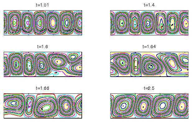
Figure 1: 32 bubbles start at time t=1.0 simultaneously equidistant on the horizontal line at y=-0.8. Ra=80000.
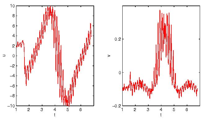
Figure 2: Fluid velocity components u and v vs. time at (0.196250 , 0.98078)
SOLUTION OF ADVECTION PROBLEMS USING h-ADAPTIVE FEM WITH DISCONTINUITY CAPTURING SUPG METHOD
Asif S. Usmani
Department of Civil and Environmental Engineering
University of Edinburgh, The Kings Buildings, Edinburgh EH9 3JN, UK
INTRODUCTION
A standard h-adaptive finite element procedure based on a-posteriori error-estimation is described.
The pure advection equation is solved using the SUPG (streamline upwind Petrov-Galerkin)
form of the finite element method. Appied to a standard benchmark problem (of
uniform flow advecting a discontinuous function) the SUPG method on its own is insufñcient
to resolve the sharp discontinuity present when used with a uniform mesh. Although the solution
is a significant improvement on other methods, it still suffers with sharp overshoots and
undershoots on either side of the discontinuity. The well-known plague of numerical models
of advection, false diffusion, is also evident downstream of the discontinuity boundary. The
h-adaptive procedure is then used in combination with the SUPG formulation and after a number
of adaptive cycles (depending upon a preset tolerance value of error) produces a high quality
solution.
ADAPTIVE STRATEGY
The adaptive strategy employed, generally follows the well established procedures developed
by Zienkiewicz and Zhu [l]. Several distinct phases of the adaptive strategy can be described
as an iterative process as follows:
- Preliminary analysis
- Recovery of the field variable gradients from the preliminary analysis. A local recovery procedure called super-convergent patch recovery [2] has been used here.
- A posteriori error estimation using the recovered gradients. The error estimator used here, was originally derived for heat conduction [3]. It is recognised that better error estimators are available for scalar advection-diffusion equations and this will be pursued in continuing this work.
- Mesh refinement based on the estimated error. Standard procedures outlined in references [1, 3] have been used.
- Data transfer to the refined mesh (for nonlinear/transient problems). Formulae given in reference [4] have been used.
- Reanalysis and back to step 2, if convergence not achieved.
THE SUPG METHOD
Introduced by Brooks and Hughes [5], this has been a very successful method for overcoming the
well known instability of standard GFEM for advection dominated problems and the excessive
dissipation of classical upwind methods. Brief details of the SUPG method are presented here.
Beginning with the weighted residual statement of the advection-diffusion equation, we have,

where,  denotes the approximated scalar variable via standard FE shape functions and v are
the advective velocities. The departure from GFEM occurs in choosing the weighting functions
as, W = N + p (against W = N in GFEM). p is a discontinuous perturbation function (see
[5] ), defined as, denotes the approximated scalar variable via standard FE shape functions and v are
the advective velocities. The departure from GFEM occurs in choosing the weighting functions
as, W = N + p (against W = N in GFEM). p is a discontinuous perturbation function (see
[5] ), defined as,

 is the so called artificial diffusion parameter. This form of p ensures that is applied only
in the streamline directions as seen by the tensorial structure of the artificial diffusion (2nd
term) in the following equation resulting from applying 2 to l, integrating the result by parts
(in standard FEM fashion) and setting W = -N, we have, is the so called artificial diffusion parameter. This form of p ensures that is applied only
in the streamline directions as seen by the tensorial structure of the artificial diffusion (2nd
term) in the following equation resulting from applying 2 to l, integrating the result by parts
(in standard FEM fashion) and setting W = -N, we have,

Application of this equation on an element level produces the FE system of algebraic equations.
The details of this and how may be calculated can be found in [5, 4]. This method was
improved further by Hughes et. al.[6] by introducing a discontinuity capturing term. This term
applies some diffusivity in the direction of the scalar gradient and reduces the phase error in
that direction. The additional term, which is added to 3, is,

 is the projection of velocity in the direction of the gradient of . The drawback of this
extra term is that it depends upon the knowledge of the temperature gradient, which makes it
nonlinear. However, it proves to be of minimal extra cost when used in an adaptive analysis
(which by its nature is iterative). The known gradients from a previous adaptive iteration are
transferred to the next mesh to use in the discontinuity capturing term. Further details on the
implementation of discontinuity capturing SUPG method can be found in [6]. is the projection of velocity in the direction of the gradient of . The drawback of this
extra term is that it depends upon the knowledge of the temperature gradient, which makes it
nonlinear. However, it proves to be of minimal extra cost when used in an adaptive analysis
(which by its nature is iterative). The known gradients from a previous adaptive iteration are
transferred to the next mesh to use in the discontinuity capturing term. Further details on the
implementation of discontinuity capturing SUPG method can be found in [6].
Benchmark problem
A widely used problem for testing advection algorithms is used. It consists of a unit square
domain with a skew velocity field (at an angle of 30|o to the horizontal here). Discontinuous
scalar values (1.0 and 0.0) are applied to the inflow boundary and negligible diffusion is specified
(10-9 here). Reference [5] shows the exact solution in comparison to the Galerkin, Quadrature
Upwind (a classical upwind FE method) and SUPG solutions. The SUPG method gives the
best results, however significant phase and dissipation errors remain. The 'converged' adap-
tive solution shown in Figure 1 shows that the discontinuity capturing operator ensures the
maximum overshoots and undershoots to remain under 3 % approximately, which produces a
numerical solution practically indistiguishable from the exact. The adaptive solution without
using discontinuity capturing also produces good results in terms of dissipation error, however
there is a maximum overshoot of approx. 11 % and maximum undershoot of approx. 12 % in
the results.

REFERENCES
- O.C. Zienkiewicz and J.Z. Zhu. A simple error estimator and adaptive procedure for practical engineering analysis. International Journal for Numerical Methods in Engineering, 24:337-357,1987.
- O.C. Zienkiewicz and J.Z. Zhu. The superconvergent patch recovery and a posteriori error estimates. Part l: The recovery technique, Part 2: Error estimates and adaptivity. International Journal for Numerical Methods in Engineering, 33:1331-1382, 1992.
- R.W. Lewis, H.C. Huang, A.S. Usmani, and J.T. Cross. Finite element analysis of heat transfer and flow problems using adaptive remeshing including application to solidification. International Journal for Numerical Methods in Engineering, 32:767-781, 1991.
- H.C. Huang and A.S. Usmani. Finite Element Analgsis for Heat Transfer - Theory and Software. Springer-Verlag, London, 1994.
- A.N. Brooks and T.J.R. Hughes. Streamline upwind/Petrov-Galerkin formulations for convection dominated flows with particular emphasis on the incompressible Navier-Stokes equations. Computer Methods in Applied Mechanics and Engineering, 32:199-259, 1982.
- T.J.R. Hughes, M. Mallet, and A. Mizukami. A new finite element formulation for computational fluid dynamics: II. Beyond SUPG. Computer Methods in Applied Mechanics and Engineeríng, 54:341-355, 1986.
THE METHOD OF LINES SOLUTION OF TIME-DEPENDENT 2-D NAVIER-STOKES EQUATIONS COUPLED WITH ENERGY EQUATION
Olcay Oymak and Nevin Selçuk
Chemical Engineering Department
Middle East Technical University, 06531 Ankara, Turkey
Flow in a pipe with sudden expansion is one of the basic problems encountered in common engineering flow systems. The separated, reattached and recirculating flow downstream of the expansion greatly influences the transport of momentum and heat. Conventional algorithms for the solution of transient two-dimensional Navier-Stokes equations consist of approximating the spatial derivatives and temporal derivatives, respectively, resulting in lower-order accuracy in time discretization. In order to alleviate this problem, another numerical technique, the method of lines (MOL) for the solution of governing partial differential equations (PDEs) is proposed. The MOL consists of converting the PDE system into an ordinary differential equation (ODE) initial value problem by discretizing the spatial derivatives together with the boundary conditions via Taylor series, Lagrange interpolation functions or weighted residual techniques, and integrating the resulting ODEs using a quality ODE solver which takes the burden of time discretization and chooses the time steps in such a way that maintains the accuracy and the stability of the evolving solution. The most important advantage of the MOL approach is that it has not only the simplicity of explicit methods but also the superiority of the implicit ones unless a poor numerical method for the solution of ODEs is used.
In this paper a novel code, developed previously for the numerical simulation of transient axisymmetric flow in a pipe with sudden expansion and validated for the prediction of developing transient flow in a pipe, was modified to incorporate the scalar transport equation for energy. The code is based on the MOL solution of time-dependent two-dimensional Navier-Stokes equations with i) an intelligent higher-order spatial discretization scheme, which chooses biased-upwind or biased-downwind discretization stencil in a zone-of-dependence manner when flow reversal occurs, and ii) a parabolic algorithm which removes the necessity of iterative solution on pressure and solution of a Poisson-type equation for the pressure. The modified code was applied for the prediction of time-development of suddenly started laminar flow in a pipe with sudden expansion with constant wall temperature. Predictions were found to show the expected trends for both unsteady and steady states. In the application of converting the PDE system into ODE initial value problem by discretizing the spatial derivatives, the convective terms should be approximated in such a way that the resulting system of ODEs should be stable according to the linear stability theory. This can only be achieved by using multi-dimensional scheme-adaptive method which is based on the choice of biased-upwind or biased-downwind points for the convective derivatives according to the sign of the coefficients (velocity components) of the concerned derivatives. Stability analysis depending on the eigenvalues of the Jacobian matrix has depicted the necessity of such an intelligent scheme in the case of flow reversal.
This paper demonstrates the ease with which the governing equations for the conservation of momentum and energy can be solved simultaneously in an accurate manner using sophisticated numerical algorithms for the solution of ordinary differential equations (ODEs). The main contribution of this study is to propose a novel code based on the MOL approach in conjunction with an intelligent higher-order spatial discretization scheme for the prediction of transient momentum and heat transfer phenomena.
Investigation of Open Boundary Treatment using Hybrid Method and Finite Element Method
Tetsuya OHASHI and Mutsuto KAWAHARA
Department of Civil Engineering,Chuo University, Tokyo,JAPAN
1. INTRODUCTION
In recent years, simulation of natural phenomena has become more and more accurate by
virtue of improvement in the performance of computers and progress in the technique of numerical
analysis. However there are some boundary problems yet to be solved. For example,
analytical solutions are influenced by accuracy of boundary conditions. Therefore it is very
important how one should treat the natural boundary condition.
 The following procedure presents a method to solve these problems. In this method the
computational value in the internal domain are connected with the general solution in the
external domain on the open boundary. Advantages of this method are that one can expect to
shorten the time of computation and to cut down the usage of computer memory, because with the
open boundary treatment there is no need to widen the analytical domain.
The following procedure presents a method to solve these problems. In this method the
computational value in the internal domain are connected with the general solution in the
external domain on the open boundary. Advantages of this method are that one can expect to
shorten the time of computation and to cut down the usage of computer memory, because with the
open boundary treatment there is no need to widen the analytical domain.
This time, the method is applied to the near-shore current analysis in this study.
But I think that this idea will be expanded to the analysis of thermal conduction.
2. BASIC EQUATION
For the governing equation, the two dimensional unsteady and nonlinear shallow water equation
is used. This can be written as follows;

where, ui is the velocity components of xi directions, g is gravity acceleration, h is water
elevation, n is coefficient of eddy viscosity, t is coefficient of undersea friction and r is density
of water. Sij is the radiation stress.
Go is the open boundary of the analytical domain.
The velocity and the water elevation are equal to general solution of external domain on the
open boundary Go.

where, symbol - means the general solution. The velocity and the water elevation are given on
the boundary GL.

where, symbol ^ means given value.
3. OPEN BOUNDARY TREATMENT
3.1 General Solution of the External Domain
General solution of the external domain is defined as follows ;

where,  are amplitude, kx, ky are the wave number of x, y directions, w is the angular
frequency and j is the imaginary number. are amplitude, kx, ky are the wave number of x, y directions, w is the angular
frequency and j is the imaginary number.
Equations (3)-(5) can be written as the following equation, looking for the eigenvalue of
which can be obtained by substituting this equations into basic equation (1),(2).

where, 
And,the wave direction is supposed three ways in this paper.
3.2 Determination of Unknown Number
The continuous condition on the open boundary is transformed as follows ;

This is multiplied by a weighting function and is integrated over the open boundary Go.

Integrating over the open boundary Go, unknown number bm can be obtained.

And, yam is the matrix of analytical solution given in equation(6), ylm is the transposed matrix
of analytical solution given in equation(6) and W'g is velocity and water elevation component
on the open boundary.
4. FINITE ELEMENT EQUATION
The basic equations(1),(2) are transformed into the following finite element equations by using
the linear interpolation function based on triangular finite elements.

Substituting equation(8) into equations(9),(10), the unknown number bm, is eliminated.
Where, M,K,H,N,S,P are the coefficient matrices respectively.
And the two-step explicit method is applied to discretize the finite element equations in
time.
5. NUMERICAL EXAMPLE
As a method of examination, numerical solutions that can be obtained by the open boundary
treatrnent were compared with one that can be obtained by giving the condition of the fixed
boundary. To examine an validity of the above-mentioned method, the following rectangle
model were used.
 The wave height and the water depth that are used as data is shown in Fig.l.
At first, the fixed boundary condition is given at all boundary in this domain.
The solution which is calculated under this condition is showed in Fig.2. And, the open boundary
treatment is performed about three cases as follows and its solutions are compared with one that
showed in Fig.2. In this calculation, the coefficient of eddy viscosity
is O.OOl m2/s, the coefficient of undersea friction is
0.1. Fig.3 are the solution under open boundary condition.

6. CONCLUDING REMARKS
In this paper, application of the Hybrid Method which is one of the open boundary treatment
in the near-shore current analysis are presented.
Until now, Hybrid Method has been applied to the analysis in which only the flow running
to the external domain from the internal one exist near the boundary like a tsunami analysis.
Therefore it was thought that the purpose of using Hybrid Method was to transmit the information
of internal domain to external one. Considering from this point, it is said that good
effect of the open boundary treatment could be verified clearly in this study. However there is
undiserable solution just as case 2 of model case in which the flow of the inside way were turned
to the opposite direction by the open boundary treatment. The cause of it is probable that
the only progressive component of the angular frequency is considered in this study. So we will
have to consider the retrogressive component to make solutions more accurate too.
Finally, it is thought that this method is effective for the analysis of the diffusion problem
like a heat transfer and we will be able to calculate more efficiently.
|
